13 Integral de fluxo de uma função sobre uma superf $\'{\i }$ cie

Seja $F$ um campo vetorial

$\mathbf{F}(x,y,z)=M(x,y,z)\mathbf{i}+N\left( x,y,z\right) \mathbf{j}+P\left( x,y,z\right) \mathbf{k}$

com $M,\ N\$ e $P$ funções escalares cont $\'{\i }$ nuas.

Integral de fluxo de $\mathbf{F}$ sobre $S:$ ${\displaystyle \iint \limits _{S}} \mathbf{F}\cdot \mathbf{\eta }dS$ onde $\mathbf{\eta }$ é o vetor normal unitário a $S$ no ponto $\left( x,y,z\right) .$ Supomos que os componentes de $\mathbf{\eta }$ $\$ são funções cont $\'{\i }$ nuas de $x,y$ e $z.$ Se $S$ é o gráfico de uma equação

$z=f\left( x,y\right)$

e fazemos $g(x,y,z)=-f(x,y)+z,$ então $S$ é também o gráfico de

$g(x,y,z)=0.$

Como $\triangledown g(x,y,z)$ é o vetor normal ao gráfico de $g(x,y,z)=0$ no ponto $\left( x,y,z\right)$ então

$\mathbf{\eta =}\frac{\triangledown g(x,y,z)}{\left\Vert \triangledown g(x,y,z)\right\Vert }=\frac{-f_{x}(x,y)\mathbf{i}-f_{y}\left( x,y\right) \mathbf{j}+\mathbf{k}}{\sqrt{1+f_{x}\left( x,y\right) ^{2}+f_{y}\left( x,y\right) ^{2}}}.$

Analogamente, há fórmulas como estas no caso em que $S$ é dado por $y=h\left( x,z\right)$ ou por $x=k\left( y,z\right) .$

Uma superf $\'{\i }$ cie $S$ é orientada $\left( \text {ou\textit{ orient\'{a}vel}}\right) ,$ se existe um vetor unitário normal $\mathbf{\eta }$ em cada ponto $\left( x,y,z\right)$ (não fronteira) e que as componentes de $\mathbf{\eta }$ são funções cont $\'{\i }$ nuas de $\left( x,y,z\right) .$ ( $\mathbf{\eta }$ varia continuamente sobre a superf $\'{\i }$ cie $S$ ). Admitamos também que $S$ tem também dois lados: o lado de cima e o lado de baixo do gráfico de $z=f\left( x,y\right) .$

Volume do prisma de área $dS$ e altura $\mathbf{F}\cdot \mathbf{\eta }$

$dV=A.h=dS\left( \mathbf{F}\cdot \mathbf{\eta }\right)$

$dV$ é a quantidade de fluido que atravessa $dS$ por unidade de tempo. Assim

$V={\displaystyle \iint \limits _{S}} \mathbf{F}\cdot \mathbf{\eta }\text { }dS$

é o volume total do flu $\'{\i }$ do que atravessa $S$ por unidade de tempo. $V$ é o fluxo de $\mathbf{F}$ através de $S.$

Definição: Fluxo do campo vetorial $\mathbf{F}$ que atravessa $S$

${\displaystyle \iint \limits _{S}} \mathbf{F}\cdot \mathbf{\eta }\text { }dS$

$m={\displaystyle \iint \limits _{S}} \delta (x,y,z)\mathbf{F}\cdot \mathbf{\eta }\text { }dS$

é a massa do flu $\'{\i }$ do que atravessa $S.$

Exemplo: Seja $S$ a parte do gráfico de $z=9-x^{2}-y^{2}$ com $z\geq 0.$ Se $\mathbf{F}(x,y,z)=3x\mathbf{i}+3y\mathbf{j}+z\mathbf{k,}$ ache o fluxo de $\mathbf{F}$ através de $S.$

Solução: Consideremos

$g(x,y,z)=z-9+x^{2}+y^{2}=0$

da $\'{\i }$

$\mathbf{\eta =}\frac{\triangledown g}{\left\Vert \triangledown g\right\Vert }=\frac{2x\mathbf{i}+2y\mathbf{j}+\mathbf{k}}{\sqrt{1+4x^{2}+4y^{2}}}$

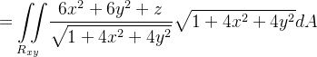
logo

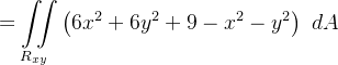
${\displaystyle \iint \limits _{S}} \mathbf{F}\cdot \mathbf{\eta }\text { }dS={\displaystyle \iint \limits _{S}} \frac{6x^{2}+6y^{2}+z}{\sqrt{1+4x^{2}+4y^{2}}}dS$

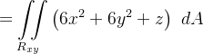
Agora

	$\displaystyle {\displaystyle \iint \limits _{S}} \frac{6x^{2}+6y^{2}+z}{\sqrt{1+4x^{2}+4y^{2}}}dS$	$\displaystyle ={\displaystyle \iint \limits _{R_{xy}}} \frac{6x^{2}+6y^{2}+z}{\sqrt{1+4x^{2}+4y^{2}}}\sqrt{1+4x^{2}+4y^{2}}dA$
	$\displaystyle$	$\displaystyle ={\displaystyle \iint \limits _{R_{xy}}} \left( 6x^{2}+6y^{2}+z\right) \ dA$

da $\'{\i }$ em coordenadas polares

	$\displaystyle {\displaystyle \iint \limits _{R_{xy}}} \left( 6x^{2}+6y^{2}+z\right) \ dA$	$\displaystyle ={\displaystyle \iint \limits _{R_{xy}}} \left( 6x^{2}+6y^{2}+9-x^{2}-y^{2}\right) \ dA$
	$\displaystyle$	$\displaystyle ={\displaystyle \iint \limits _{R_{xy}}} \left( 9+5x^{2}+5y^{2}\right) \ dA$
	$\displaystyle$	$\displaystyle =\int _{0}^{2\pi }\int _{0}^{3}\left( 9+5r^{2}\right) rdrd\theta =\frac{567}{2}\pi .$

13 Integral de fluxo de uma função sobre uma superfcie

13 Integral de fluxo de uma função sobre uma superf $\'{\i }$ cie